
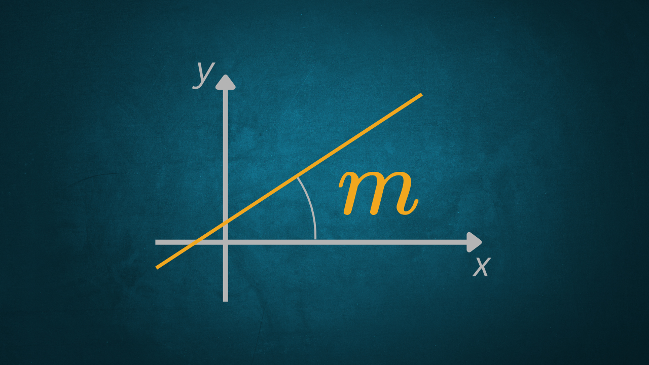
The slope is one of the central concepts in analytic geometry. Geometrically, it describes how inclined a line is in the coordinate plane; analytically, it provides essential information for working with a line’s equation.
Understanding what slope means and how to calculate it makes it possible to read a line’s equation correctly and to use it appropriately and with confidence when studying its properties and solving problems and exercises.
This article works through slope systematically, from its geometric meaning to a step-by-step calculation, supported along the way by worked examples, interactive graphs, and a look at the special cases. The goal is to provide a solid, coherent foundation for studying lines with method and precision.
What Is the Slope of a Line
The slope is a quantity associated with a line in the coordinate plane that describes its inclination relative to the x-axis. It gives essential information about how a line sits in the coordinate plane, and about the “behavior” of its coordinates.
Geometrically, the slope tells us whether a line is increasing, decreasing, or horizontal, and measures how quickly the y-coordinate changes as the x-coordinate changes. Analytically, it’s one of the fundamental parameters that characterizes a line’s equation, linking its graphical representation to its algebraic expression.
In this sense, the slope is a structural piece of information about the line — one that’s essential for interpreting its equation and studying its properties.
Definition of Slope
Given a line \(r\), the slope of \(r\) is defined as the constant parameter \(m\), given by the ratio between the change in the y-coordinate per unit change in the x-coordinate. In formulas:
with
In light of this definition, a few observations follow right away:
- If \(m>0\), the line is increasing (as \(x\) increases, \(y\) increases too)
- If \(m<0\), the line is decreasing (as \(x\) increases, \(y\) decreases)
- If \(m=0\), the line is horizontal
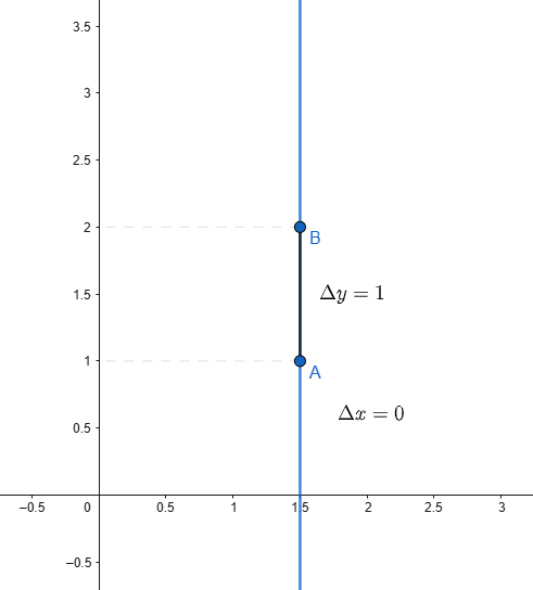
- If the line is vertical (parallel to the \(y\)-axis), the slope is undefined
In other words, the slope tells us how quickly a line rises or falls vertically as \(x\) changes.
The examples that follow will help make the ideas of an increasing, decreasing, horizontal, and vertical line clearer, along with how each one connects to the slope.
Calculating the Slope
If two distinct points with coordinates \((x_1,y_1)\) and \((x_2, y_2)\) are known in the coordinate plane, the slope can be calculated as:
Example 1
Given the points \(A(0,1)\) and \(B(3,7)\), find the slope of the line through these points. Then find the line’s equation in slope-intercept form.
SOLUTION
Applying (2) gives the solution directly:
Finally, to find the line’s equation in slope-intercept form \((y=mx+b)\), notice that point \(A\) lies on the y-axis, so the y-coordinate of \(A\) is exactly \(b\). In formulas:
Substituting into the slope-intercept form gives:
Example 2
Given the points \(C(-2,4)\) and \(D(1,-2)\), find the slope of the line through these points. Then find the line’s equation in slope-intercept form.
SOLUTION
Applying (2) again, this time gives:
To find the line’s equation, following the same steps as in Example 1:
so, simplifying,
The slope-intercept equation of the line therefore turns out to be:
Geometric Meaning of Slope
In this section, we’ll bring out the relationship between a line’s slope and its inclination. The two quantities are, in fact, closely connected.
INCREASING LINE
Consider, as an example, points A and B with known coordinates that lie on the line \(y=x/2\), as shown in Fig.1.
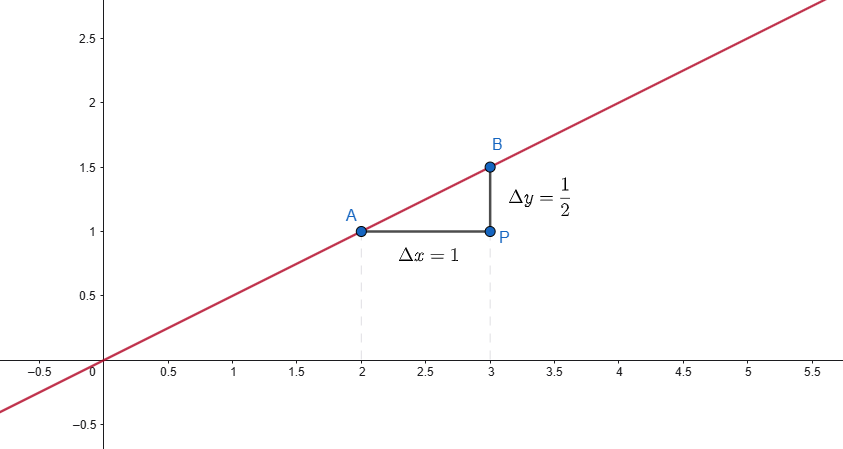
Specifically, the coordinates of the points are \(A(2,1)\) and \(B(3,3/2)\).
Calculating the increments gives:
Now applying definition (1) of slope:
which is positive.
Let’s take this further to the general case. Whenever the slope \(m\) turns out to be greater than zero, the increase in \(y\)-coordinates and the increase in \(x\)-coordinates will move in the same direction. In formulas:
Put another way:
which means the line is increasing (Fig.1).
⚠️ The slope can therefore be interpreted as the change in the y-coordinate when the change in the x-coordinate is one unit — but with one clarification: in practice (especially when solving exercises), the calculated change in \(x\) doesn’t need to be exactly one unit. Since the slope of a line is a constant parameter, it can always be calculated as the ratio between the change in \(y\) and the change in \(x\), even when that change in \(x\) isn’t equal to one.
DECREASING LINE
Consider, as an example, points A and B with known coordinates that lie on the line \(y=-\frac{x}{3}\), as shown in Fig.2.
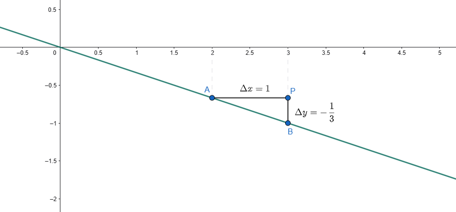
Specifically, the coordinates of the points are:
Calculating the increments gives:
Now applying definition (1) of slope:
which is negative.
The same reasoning applies here, now for a negative slope. When the slope \(m\) is less than zero, the increase in \(y\)-coordinates and the increase in \(x\)-coordinates will move in opposite directions. In formulas:
Put another way:
which means the line is decreasing (Fig.2).
Special Cases: Horizontal and Vertical Lines
Horizontal lines (parallel to the \(x\)-axis) and vertical lines (parallel to the \(y\)-axis) are two special cases when it comes to calculating the slope. We’ll show that in the first case, the slope always comes out to zero, while in the second case, the slope isn’t defined at all and therefore can’t be calculated.
Horizontal Lines
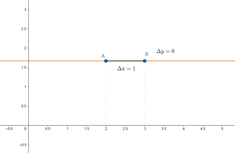
On a horizontal line, every point on the line has the same y-coordinate. As a result, no matter how the x-coordinate changes, the change in the y-coordinate is always zero \((\Delta y=0)\).
Given this, applying definition (1) and setting \((\Delta y=0)\) gives:
from which it immediately follows that
We can conclude that every line of the form \(y=k\) (horizontal lines) has a slope of zero. In formulas:
Vertical Lines
On a vertical line, every point on it has the same x-coordinate. So, regardless of how the y-coordinate changes, the change in the x-coordinate will always be zero.
However, notice that in this particular case the denominator of (1) would become zero which makes the ratio undefined.
We can conclude, then, that for a vertical line (with the general equation \(x=h\)), the slope isn’t defined.
In formulas:
Slope and the Forms of a Line’s Equation
Slope-Intercept Form
In the slope-intercept form of a line’s equation, the slope \(m\) appears directly within the equation:
- \(m\) = slope
- \(b\) = y-intercept
Once the value of \(m\) and the y-intercept \(b\) are known, the line’s equation can be written down immediately.
Example: \(m=−1\), \(b=4\) → \(y=−x+4\)
Standard Form
In the standard form of a line’s equation, unlike the slope-intercept form, the slope doesn’t appear directly. The standard form is written as:
with \(B\neq0\).
Even so, this equation can be rewritten in slope-intercept form through the following steps:
- Rewriting in slope-intercept form: \(y=-\frac{A}{B}x + \frac{C}{B}\)
- Slope: \(−A/B\)
Example:
from which
Parametric Form
A line can also be represented in what’s known as parametric form, as a real parameter \(t\) varies. It’s written as:
In this case, the slope is directly tied to these direction parameters, and equals: \(m=b/a\), provided \(a\neq 0\).
⚠️ Here, \(a\) and \(b\) are the components of the direction vector — a different \(b\) from the y-intercept \(b\) used above in slope-intercept form.
Example
Slope and Parallel/Perpendicular Lines
- Two parallel lines have the same value of the slope \(m\)
- Two perpendicular lines have slopes that are the negative reciprocal of one another. In formulas: \(m_1 \cdot m_2 = -1\)
Numerical example:
- Given the line \(r\): \(y=3x+2\) → \(m=3\)
- An example of a line \(s\) parallel to \(r\): \(y=3x−1\)
- An example of a line \(z\) perpendicular to \(r\): \(y=-\frac{1}{3}x + 4\)
Interactive Graph
Below is the interactive graph of a generic line with variable slope, passing through the point with coordinates \((3,1)\).
Point on the line: x = 3, y = 1
Common Mistakes
- Confusing \(Δy/Δx\) with \(Δx/Δy\)
- Applying the slope formula to vertical lines as well
- Confusing the slope with the y-intercept \(b\)
Practical Applications
The concept of slope comes up in a wide range of contexts, including, for example:
- Linear modeling in physics and economics
- Analyzing inclines (roads, ramps)
- Building the groundwork for more complex geometry problems
For the complete picture of how slope fits into the broader study of lines — equations, parallelism, perpendicularity, and more — see the dedicated guide on the line in analytic geometry.
Conclusion
The slope isn't just a number: it points to the direction of a line and shows how closely algebra and geometry are tied to one another. Understanding it thoroughly makes it possible to read lines graphically, compare them, and understand relationships between them, such as parallelism and perpendicularity.
This understanding naturally connects to other mathematical topics: it makes it possible, for example, to link lines to linear functions, to analyze rates of change, and to grasp more advanced ideas such as slopes in three-dimensional analytic geometry, max/min problems in calculus, and much more.
Final Test
Below is a short quiz to check understanding of the slope of a line: its definition, calculation, special cases, and the different equation forms covered in this article.
Cite this resource
"This page didn't write itself — every word here was written and checked by hand. If it helped you, sharing it or citing it as a source helps it reach the next student who needs it."
Citation
HTML link to copy