
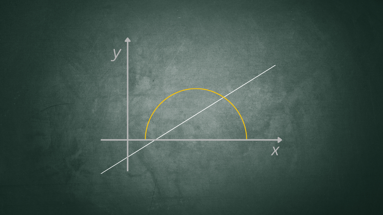
In the study of analytic geometry, the circle is not limited to representing a geometric locus — it also becomes an interpretive tool for tackling problem types that, on the surface, belong to algebraic analysis. Among these problems, radical inequalities occupy a place of particular importance.
When a radical inequality contains an expression of the form \(\sqrt{r^2-x^2}\), it is possible to recognize the graph of a semicircle associated with the corresponding circle centered at the origin with radius \(r\), described by the equation \(x^2+y^2=r^2\).
This article presents a graphical method whose purpose is to solve a radical inequality, transforming it into a geometric problem in the process. Solving the inequality will turn out to be equivalent to determining the values of \(x\) for which the graph of one function (for example, a line) lies above or below another (a semicircle). This approach does not replace the algebraic method — it complements it in a meaningful way, making the significance of the solutions visible and reducing the risk of errors tied to manipulating radicals.
This method builds a bridge between the study of radical inequalities and the analytic geometry of the circle.
What follows includes both the theory and a series of worked examples in increasing order of difficulty, from the simplest cases up to more elaborate ones involving two semicircles and functions with absolute value.
The Method for Graphically Solving Radical Inequalities
The graphical method for solving radical inequalities rests on the following general principle:
given an inequality of the form:
\[f(x) \gtrless g(x)\]
where \(f\) and \(g\) are real functions of a real variable, the solution is obtained by determining the set of \(x\)-values for which the graph of \(f\) lies, respectively, above or below the graph of \(g\).
In particular, for a radical inequality of the form
\[\sqrt{r^2-x^2} \gtrless g(x)\]
the procedure begins by identifying:
- \(y = \pm \sqrt{r^2-x^2}\): the upper (or lower) semicircle centered at \(O(0,0)\) with radius \(r\), defined for \(x \in [-r, r]\)
- \(y=g(x)\): the second function (a line, a semicircle, an absolute value, and so on)
Operational procedure for graphically solving radical inequalities
The method unfolds in three stages:
Stage 1 — Determining the domain. The radical function \(\sqrt{r^2-x^2}\) is defined for \(r^2-x^2 \geq 0\), that is, for \(x \in [-r, r]\). The domain of the inequality therefore coincides with this interval, intersected with the domain of the other function (\(g(x)\)).
Stage 2 — Computing the intersections. Solve the system:
\[\begin{cases} y = \sqrt{r^2-x^2} \\ y = g(x) \end{cases}\]
whose solutions give the points at which the two graphs, if any, intersect.
Stage 3 — Analyzing the relative position. Using the graph, or by numerical verification, determine which of the two graphs lies above the other on the intervals determined by the intersection points. The solution of the inequality corresponds to the union of the intervals on which the required relation holds.
Worked Examples
In the following worked examples, the graphical method is applied to several types of radical inequalities, in increasing order of difficulty.
Example 1 — Semicircle and Line (Base Case)
Solve the following inequality graphically:
\[\sqrt{1-x^2} < x + 1\]
SOLUTION
Set \(y=\sqrt{1-x^2}\) under the condition \(y\geq0\), since the radical must necessarily be non-negative.
Squaring both sides gives
\[y^2=1-x^2\]
and therefore
\[x^2+y^2=1\]
which, subject to the constraint above (\(y\geq0\)), represents the equation of a semicircle centered at the origin with unit radius, lying in the first and second quadrants.
Now consider the function
\[y=x+1\]
which represents the right-hand side of the given inequality. This gives the graph shown below (Fig. 1):
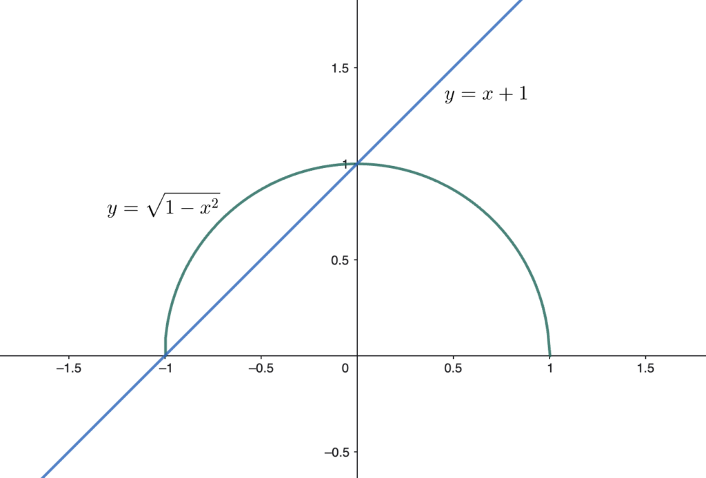
Solving the inequality therefore amounts to determining the interval of \(x\)-values for which the values taken by the function \(y=\sqrt{1-x^2}\) are smaller than the values of the line (\(y=x+1\)) at the same \(x\)-coordinate.
This condition holds only on the interval of \(x\)-values such that
\[x\in \left(0,1 \right]\]
Note that the point with \(x\)-coordinate \(x=0\) is excluded from the solution interval, since the inequality is strict, while for \(x>1\) the semicircle is not defined (its domain being the interval \([-1,1]\)).
Example 2 — Semicircle and Line Through the Origin
Solve the following inequality graphically:
\[\sqrt{4-x^2} \geq x\]
SOLUTION
The first step, needed for the radical to make sense, is to require the radicand to be non-negative, in formulas:
\[4-x^2 \geq0\]
Solving this inequality gives:
\[x^2-4\leq0\]
with associated equation:
\[x^2-4=0 \rightarrow x=\pm{2}\]
The inequality \(x^2-4\leq0\) therefore holds on the closed interval \(x \in [-2,2]\).
Note also that the left-hand side of the given inequality represents the function
\[y=\sqrt{4-x^2}\]
which coincides with the semicircle lying in the first and second quadrants, associated with the circle
\[y^2=4-x^2\]
centered at the origin with radius \(\sqrt{4}=2\), subject to the constraint \(y\geq0\).
Turning now to the right-hand side of the given inequality, consider the function
\[y=x\]
which is the bisector of the first and third quadrants.
Solving the original inequality is essentially equivalent to finding the interval of \(x\)-values for which the semicircle is greater than or equal to the line \(y=x\).
Plot both functions on the same graph (Fig. 2).
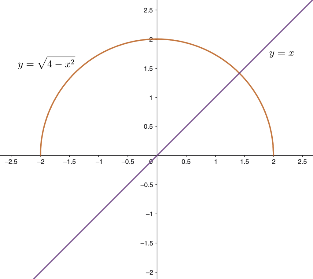
The graph shows that to find the solution, the intersection point between the circle and the line must first be located by setting up the system of the two functions. Thus:
\[\begin{cases} x^2+y^2=4 \\ y = x \end{cases}\]
subject to \(y \geq0\).
Substituting the second equation into the first gives
\[x^2+x^2=4\] \[2x^2=4\] \[x^2=2\] \[x=\pm \sqrt{2}\]
The graph shows that the only admissible solution is
\[x=+\sqrt{2}\]
with corresponding \(y\)-coordinate at the intersection point \(y=+\sqrt{2}>0\).
Conversely, for \(x=-\sqrt{2}\) the \(y\)-coordinate of the intersection point on the circle would be \(y=-\sqrt{2}\), so that solution is not admissible.
In light of these considerations, and taking the original inequality into account, we conclude that the \(y\)-coordinates of the semicircle are greater than or equal to the \(y\)-coordinate of the line, at corresponding values of \(x\), on the interval of values such that
\[x \in [-2, \sqrt{2}]\]
Example 3 — Two Semicircles
Solve the following radical inequality graphically
\[\sqrt{9-x^2} > \sqrt{-x^2 + 4x}\]
SOLUTION
Here, two semicircles must be compared:
- \(y_1 = \sqrt{9-x^2}\): upper semicircle centered at \(O(0,0)\) with radius 3;
- \(y_2 = \sqrt{-x^2+4x}\): upper semicircle centered at \(C(2,0)\) with radius 2;
Now construct the graph of both circles (Fig. 3).
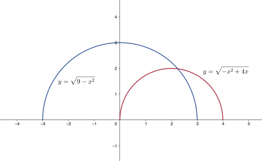
The graph clearly shows that the semicircle \(y=\sqrt{9-x^2}\) is defined on the interval \(-3 \leq x \leq 3\), while the semicircle \(y=\sqrt{-x^2+4x}\) is defined on the interval \(0 \leq x \leq 4\). Valid solutions will therefore be sought only where both curves exist, that is, on the interval \(0 \leq x \leq 3\).
The graph immediately shows that the semicircle \(y_1\) remains greater than \(y_2\) on the interval of \(x\)-values between the origin and their intersection point.
To find the intersection point of the two semicircles, it suffices to solve the system formed by the associated circles and eliminate one of the two variables, then choose the solution consistent with the graph (in this case, positive, since the intersection lies in the first quadrant).
Carrying out the computation:
\[\begin{cases} x^2+y^2=9 \\ x^2+y^2-4x=0 \end{cases}\]
Subtracting one equation from the other (the most direct operation in this case) gives
\[4x=9\]
so that
\[x=\frac{9}{4}\]
The solution of the inequality is therefore the interval of \(x\)-values such that
\[x \in [0,\frac{9}{4})\]
Example 4 — Semicircle and Absolute Value
Solve the following radical inequality graphically
\[\sqrt{1-x^2} \leq |x|\]
SOLUTION
Here, the upper semicircle of radius 1 must be compared with the absolute value function:
- \(y_1 = \sqrt{1-x^2}\): upper semicircle centered at \(O(0,0)\) with radius 1;
- \(y_2 = |x|\).
Now construct the graph (Fig. 4).
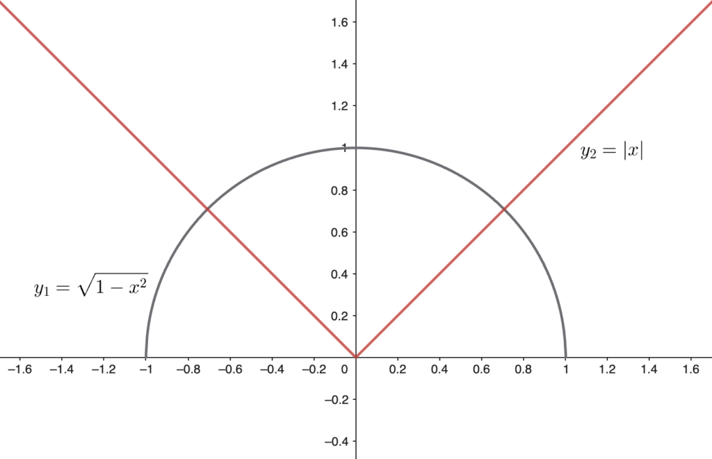
Looking at Fig. 4, notice first that the function \(y_2=|x|\) is defined for every \(x\), while the semicircle \(y_1=\sqrt{1-x^2}\) is defined on the closed interval \([-1,1]\); consequently, any \(x\)-values solving the radical inequality must be sought exclusively within that interval.
The graph also shows that the function \(y_2\) remains greater than \(y_1\) for \(x\) between -1 (included) and the \(x\)-coordinate of the intersection of the two functions in the second quadrant, together with the symmetric interval with respect to the \(y\)-axis.
Find the intersection point between \(y_1\) and \(y_2\), keeping in mind that the latter equals
\[y_2=-x \quad \text{for} \quad x<0 \]
This gives the system
\[\begin{cases} y=\sqrt{1-x^2} \\ y=-x \end{cases}\]
subject to \(y\geq0\). Solve the system by first squaring the first equation and then eliminating \(y\):
\[\begin{cases} y^2=1-x^2 \\ y=-x \end{cases}\]
\[\begin{cases} x^2+y^2=1 \\ y=-x \end{cases}\]
Square the second equation and rewrite the first as follows:
\[\begin{cases} x^2+y^2=1 \\ y^2=(-x)^2=x^2 \end{cases}\]
Substituting the second into the first (eliminating \(y\)) gives
\[x^2+x^2=1\] \[2x^2=1\] \[x=\pm \frac{1}{\sqrt{2}}\]
Only the negative solution should be kept (the positive one falls in the fourth quadrant, where \(y<0\), contrary to the hypothesis).
By an analogous argument, it can easily be shown that the intersection between the semicircle and the function \(y_2=|x|\) for \(x>0\) gives, as the only acceptable solution,
\[x=\frac{1}{\sqrt{2}}\]
The solution of the inequality is therefore the interval of \(x\)-values such that
\[x\in\left[-1,-\frac{1}{\sqrt{2}}\right]\cup\left[\frac{1}{\sqrt{2}},1\right]\]
Example 5 — Absolute Value with Semicircle (Advanced)
Solve the following inequality graphically
\[|4-\sqrt{36-x^2}|<x-3\]
SOLUTION
For the radical to make sense, it is required that
\[36-x^2 \geq0\]
which, as known from the theory of quadratic inequalities, has solution
\[-6 \leq x \leq 6\]
Note further that the right-hand side quantity \((x-3)\) must be positive, being greater than an absolute value, in formulas:
\[x-3 > 0\] so that \[x > 3\]
The possible solutions of the inequality must therefore be sought on the interval
\[3<x\leq6\]
Since this is a graphical solution procedure for the inequality, it is convenient at this point to plot the graphs of the following functions:
\[y_1=|4-\sqrt{36-x^2}|\]
\[y_2=x-3\]
In particular, with regard to the function \(y_1\), note that it equals
\[y_1=\begin{cases} 4-\sqrt{36-x^2} \quad \text{for} \quad 4-\sqrt{36-x^2}>0 \\ -4+\sqrt{36-x^2} \quad \text{for} \quad 4-\sqrt{36-x^2}<0 \\ 0 \quad \text{for} \quad 4-\sqrt{36-x^2}=0 \end{cases}\]
Now find the intersections of \(y_1\) with the \(x\)-axis, that is, solve the equation
\[\quad 4-\sqrt{36-x^2}=0\]
which, working through the steps, gives:
\[\quad 4=\sqrt{36-x^2}\] \[16=36-x^2\] \[x^2=20\] \[x_{1,2}=\pm 2\sqrt{5}\]
Taking these solutions into account, \(y_1\) can be rewritten as
\[y_1=\begin{cases} 4-\sqrt{36-x^2} \quad \text{for} \quad -6 \leq x<-2\sqrt{5} \vee 2\sqrt{5}<x \leq 6 \\ -4+\sqrt{36-x^2} \quad \text{for} \quad -2\sqrt{5}<x<2\sqrt{5} \\ 0 \quad \text{for} \quad x=\pm 2\sqrt{5} \end{cases}\]
The two functions \(y_1\) and \(y_2\) are shown separately below (Fig. 5).
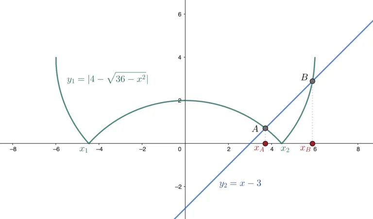
Fig. 5 clearly shows that the line \(y_2=x-3\) is greater than \(y_1=|4-\sqrt{36-x^2}|\) on the interval
\[x_A<x<x_B\]
where \(x_A\) is the \(x\)-coordinate of the intersection between the line and the arc of the circle corresponding to the interval \(x_1,x_2\). To find \(x_A\), the following system must be solved:
\[\begin{cases} y=-4+\sqrt{36-x^2} \quad \text{for} \quad -2\sqrt{5}<x<2\sqrt{5} \\ y=x-3 \quad \\ y>0 \end{cases}\]
Making the substitutions
\[x-3=-4+\sqrt{36-x^2}\] \[x+1=\sqrt{36-x^2}\]
then squaring and simplifying gives
\[2x^2+2x-35=0\]
which, when solved, gives
\[x=\frac{-1\pm\sqrt{71}}{2}\]
whose only acceptable solution is the positive one, since the intersection must lie in the first quadrant. It follows that
\[x_A=\frac{-1+\sqrt{71}}{2}\]
To obtain the intersection \(x_B\), proceed similarly, keeping in mind that this time the system to be solved is
\[\begin{cases} y=4-\sqrt{36-x^2} \quad \text{for} \quad -6 \leq x<-2\sqrt{5} \vee 2\sqrt{5}<x \leq 6 \\ y=x-3 \quad \\ y>0 \end{cases}\]
which gives
\[x-3=4-\sqrt{36-x^2}\] \[x-7=-\sqrt{36-x^2}\]
then, squaring again and simplifying, this gives
\[2x^2-14x+13=0\]
which, when solved, gives the following solutions
\[x=\frac{7\pm\sqrt{23}}{2}\]
this time both positive.
The acceptable solution must still lie in the first quadrant; consequently, noting that the \(y\)-coordinate values corresponding to the \(x\)-values found equal
\[y(\frac{7+\sqrt{23}}{2})=\frac{7+\sqrt{23}}{2}-3=\frac{1+\sqrt{23}}{2}\approx 2.90\] \[y(\frac{7-\sqrt{23}}{2})=\frac{7-\sqrt{23}}{2}-3=\frac{1-\sqrt{23}}{2}\approx -1.90\]
the valid solution must be
\[x_B=\frac{7+\sqrt{23}}{2}\]
The original inequality is therefore satisfied on the interval
\[\frac{-1+\sqrt{71}}{2}<x<\frac{7+\sqrt{23}}{2}\]
Common Mistakes
When applying the graphical method to inequalities involving semicircles, the most frequent errors mainly concern domain handling, graph interpretation, and the use of squaring.
A first mistake consists of overlooking the domain of the radical function. The function \(y = \sqrt{r^2-x^2}\) is defined only for \(-r \le x \le r\), and this interval represents the only portion on which the semicircle exists. Any value outside it cannot be a solution, even if it was correctly obtained from a purely algebraic standpoint. When multiple radicals are present, the correct domain is given by the intersection of the individual intervals of definition.
Another mistake concerns the step of squaring to determine intersection points. Solving an equation of the form \(\sqrt{r^2-x^2} = ax + b\) implicitly introduces the condition that the right-hand side be non-negative. If this condition is not checked, solutions may be obtained that do not satisfy the original equation. This point remains important in the graphical method as well, since the intersection points must be consistent with the conditions of the problem.
From an interpretive standpoint, it is common to confuse the direction of the inequality with the relative position of the graphs. The inequality is satisfied on the intervals where the semicircle lies above or below the line, depending on the sign. A hasty reading of the graph can lead to reversing this relationship; for this reason, it is always useful to check at least one value in each interval identified.
A further difficulty concerns handling the domain endpoints and intersection points. At the endpoints of the interval, the semicircle does not always take the value zero, and those endpoints do not necessarily belong to the solution set. The same holds for intersection points.
Finally, in some cases the functions involved exhibit symmetries that are also reflected in the solution; failing to recognize them can lead to incomplete results.
Overall, the graphical method is highly effective, but it requires care in correctly connecting domain, intersections, and graph interpretation. When these three aspects are handled correctly, errors are significantly reduced.
Conclusion
The graphical method for radical inequalities with semicircles is an example of how analytic geometry can offer interpretive tools for problems of an algebraic nature. Recognizing the graph of a semicircle in \(\sqrt{r^2-x^2}\) is not merely a formal observation — it is the first step toward turning a radical inequality into a problem about the relative position of curves, more intuitive and less prone to the typical errors of the purely algebraic method.
The domain, the intersections, and the graphical sign analysis are the three stages that structure every solution: mastering them provides a systematic method applicable to a wide range of radical inequalities and, with appropriate modifications, extendable to comparisons between any pair of functions in the coordinate plane.
This technique is one part of a larger toolkit: the complete guide to the circle in coordinate geometry covers the rest, from tangent lines to pencils of circles and more.
Cite this resource
"If this explanation saved you some confusion, passing it along costs you nothing and might save someone else the same struggle."
Citation
HTML link to copy