
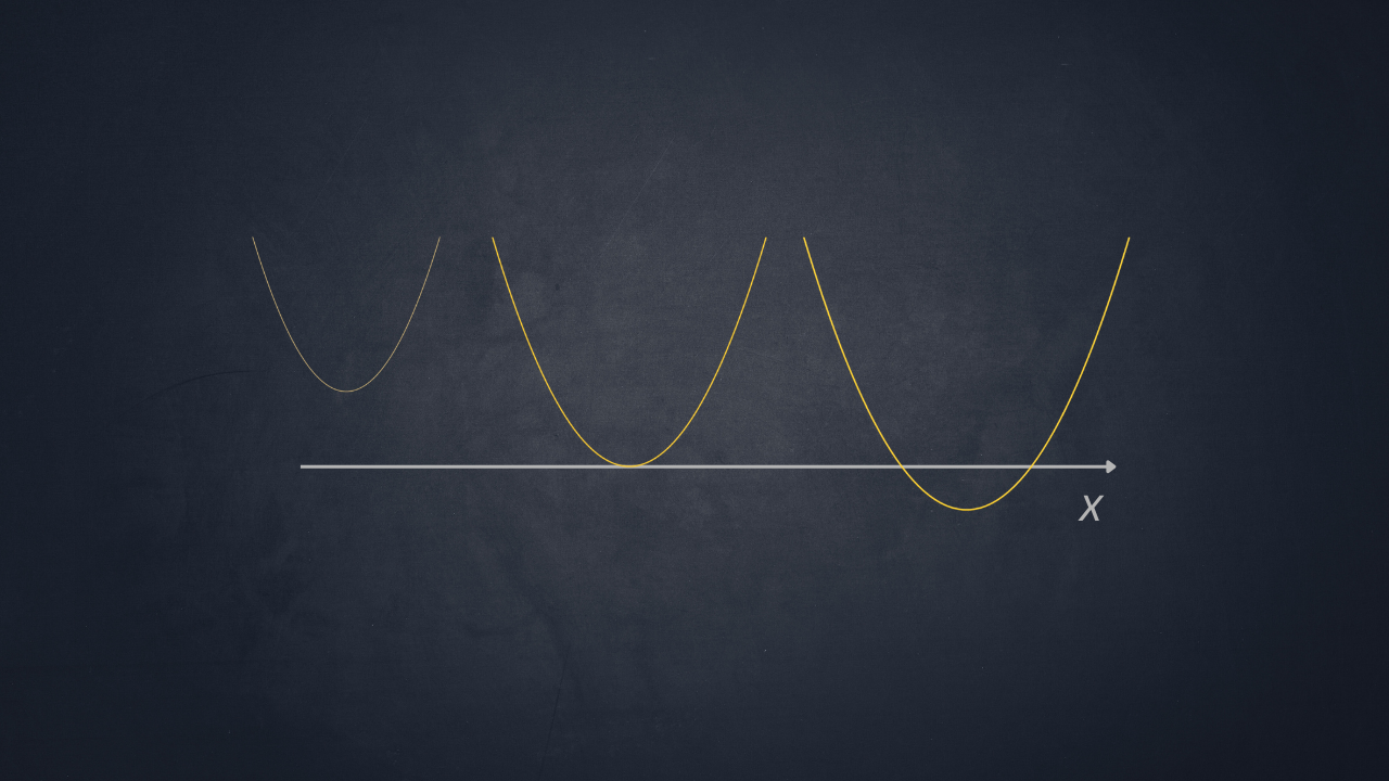
The graphical method makes it possible to interpret an equation or an inequality through the graph of one or more functions, turning an algebraic problem into a geometric one. For quadratic equations, this interpretation is particularly direct: the solutions correspond to the intersections between a parabola and the x-axis, or to the intersections between two general quadratic functions.
This article shows how to use the graphical method to solve quadratic equations and inequalities, examining the geometric meaning of the solutions and the role of the discriminant. Several examples are also presented in which the graph makes it possible to find the solutions quickly and, in more involved cases, the reading of the graph is complemented by an analytical check.
Solving a Quadratic Equation Graphically
Given a quadratic equation of the form
\[ax^2+bx+c=0 \tag{1}\]
it can be interpreted, in a completely equivalent way, as the equation arising from the system
\[\begin{cases} y=ax^2+bx+c \\ y=0 \end{cases} \tag{2}\]
In essence, solving equation (1) amounts to finding the intersections, if any, between the parabola and the x-axis (\(y=0\)). Put differently, solving (1) amounts to finding the points of the parabola \(y=ax^2+bx+c\) whose y-coordinate is zero, if any exist.
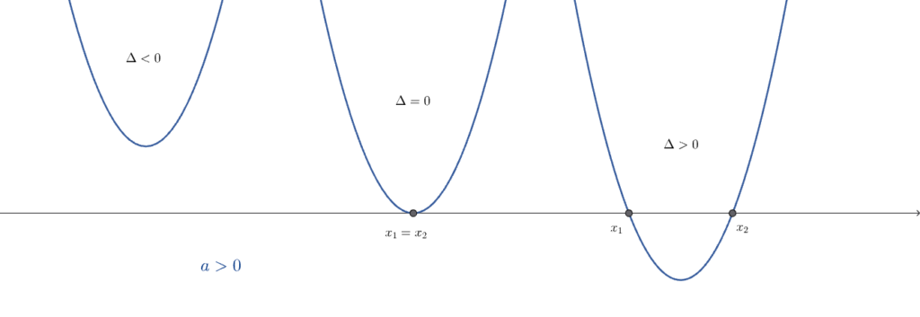
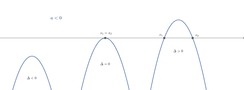
Figs. 1 and 2 show clearly that:
- if \(\Delta>0\), the parabola intersects the x-axis at two distinct points, with x-coordinates \(x_1\) and \(x_2\);
- if \(\Delta=0\), the parabola is tangent to the x-axis at a single point, with \(x_1=x_2\);
- if \(\Delta<0\), the parabola has no real intersection with the x-axis.
Example 1
Solve the following quadratic equation graphically: \(-x^2+5x-4=0\).
SOLUTION
The given equation can be put immediately in the form of system (2):
\[\begin{cases} y=-x^2+5x-4 \\ y=0 \end{cases}\]
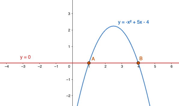
Consequently, solving the given equation consists of finding the intersections between the parabola \(y=-x^2+5x-4\) and the line representing the x-axis (with equation \(y=0\)).
These intersections are found by solving system (2) as follows:
\[-x^2+5x-4=0\]
from which
\[\Delta=b^2-4ac=5^2-4(-1)(-4)=9\]
\[x_{1,2}=\frac{-b\pm\sqrt{\Delta}}{2a}=\frac{-5\pm3}{-2}\]
\[x_1=1\]
\[x_2=4\]
Fig. 3 shows the solutions in graphical form, namely the intersections between the parabola and the x-axis.
Example 2
Solve the following equation graphically:
\[\sqrt{1-x^2}=\sqrt{x}\]
SOLUTION
The given equation can be written as
\[\begin{cases} y=\sqrt{1-x^2} \\ y=\sqrt{x} \end{cases}\]
and then, squaring both sides and rearranging,
\[\begin{cases} x^2+y^2=1 \quad y\geq0 \\ x=y^2 \quad y\geq0 \end{cases}\]
Caution: since both radicals appearing in the system must be nonnegative, the constraint \(y\geq0\) must be imposed at the same time as the squaring.
The first equation in the last system, subject to the constraint \(y\geq0\), represents the upper semicircle (lying in the first and second quadrants) centered at the origin with radius 1. The second equation represents the portion of a parabola with a horizontal axis that lies in the first quadrant.
Fig. 4 shows more clearly what happens from the graphical point of view.
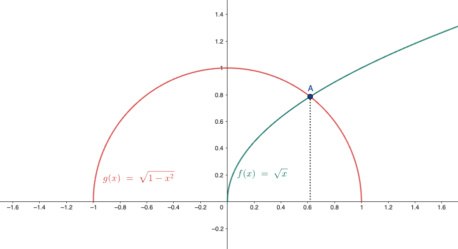
Fig. 4 clearly shows that the equation has only one solution.
Let us now determine it analytically.
The system
\[\begin{cases} x^2+y^2=1 \quad y\geq0 \\ x=y^2 \quad y\geq0 \end{cases}\]
can simply be rearranged as
\[\begin{cases} x^2+y^2-1=0 \quad y\geq0 \\ x-y^2=0 \quad y\geq0 \end{cases}\]
and then, adding the two equations term by term, we obtain:
\[x^2+x-1=0\]
from which
\[x_{1,2}=\frac{-1\pm\sqrt{5}}{2}\]
Comparing the solutions obtained with the graph in Fig. 4 shows that the only acceptable solution is the positive one:
\[x_1=\frac{-1+\sqrt{5}}{2}\approx0.618\]
It is also worth noting that
\[x_2=\frac{-1-\sqrt{5}}{2}<0\]
cannot possibly be a solution. Indeed, from the analytical point of view, since the equation \(x=y^2\) must be satisfied, the absurd result
\[x_2=y^2<0\]
would follow, since a square cannot be negative. Consequently, \(x_2\) is not a solution of the given equation.
Solving a Quadratic Inequality Graphically
Consider a quadratic inequality of the form
\[ax^2+bx+c>0 \tag{3}\]
It can be interpreted, in a completely equivalent way, as the following system consisting of an equation and an inequality:
\[\begin{cases} y=ax^2+bx+c \\ y>0 \end{cases} \tag{4}\]
In essence, solving inequality (3), in the formulation (4), amounts to finding the points of the parabola \(y=ax^2+bx+c\) with positive y-coordinate (\(y>0\)).
Looking again at Figs. 1 and 2, the following can be observed.
For \(a>0\), the parabola opens upward (Fig. 1), and the following cases arise:
- if \(\Delta>0\), the parabola is positive for \(x<x_1\) or \(x>x_2\) (where \(x_1<x_2\));
- if \(\Delta=0\), the parabola is tangent to the x-axis at a single point, so it is positive everywhere except at \(x_1=x_2\), where it equals zero;
- if \(\Delta<0\), the parabola has no real intersection with the x-axis and is always positive. In this case, system (4) has a solution for every \(x\).
For \(a<0\), the parabola opens downward (Fig. 2), and the following cases arise:
- if \(\Delta>0\), the parabola is positive for \(x_1<x<x_2\);
- if \(\Delta=0\), the parabola is tangent to the x-axis at a single point, so it is negative everywhere except at \(x_1=x_2\), where it equals zero;
- if \(\Delta<0\), the parabola has no real intersection with the x-axis and is always negative. In this case, system (4) has no real solution.
Note: the above applies to the search for solutions with \(y>0\); however, the same reasoning extends to other cases, for example the search for solutions with \(y<0\), by adapting the conclusions accordingly.
Example 1
Solve the quadratic inequality \(x^2-3<0\) graphically.
SOLUTION
This amounts to solving a system consisting of an equation and an inequality:
\[\begin{cases} y=x^2-3 \\ y<0 \end{cases}\]
The equation \(y=x^2-3\) represents a parabola with a vertical axis, with vertex at the point with coordinates \((0,-3)\), that opens upward (\(a>0\)) (see Fig. 5).
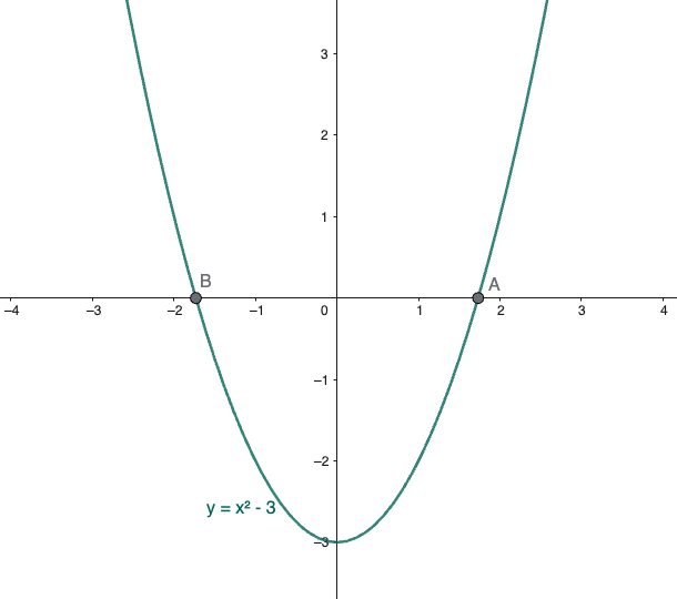
Since the system must also satisfy the inequality \(y<0\), the set of solutions consists of the values of \(x\) for which the y-coordinate of the parabola is negative, that is, graphically, the interval of x-coordinates between points \(B\) and \(A\).
It remains to determine the numerical values of the x-coordinates of these points. This is very simple, since they are points of the parabola with zero y-coordinate and therefore must satisfy its equation for \(y=0\), that is:
\[x^2-3=0\]
which, once solved, gives
\[x_{1,2}=\pm\sqrt{3}\]
from which the coordinates of the points follow:
\[A(\sqrt{3},0)\]
\[B(-\sqrt{3},0)\]
The solution of the problem is therefore
\[-\sqrt{3}<x<\sqrt{3}\]
Example 2
Solve the following inequality graphically:
\[x^2-x>4-2x\]
SOLUTION
The inequality represents the system:
\[\begin{cases} f(x)=x^2-x \quad \text{(parabola)} \\ g(x)=4-2x \quad \text{(line)} \\ f(x)>g(x) \end{cases}\]
In other words, the question is for which set of values of \(x\) the parabola \(f(x)\) takes values greater than the line \(g(x)\). This situation can be shown immediately in graphical form (see Fig. 6).
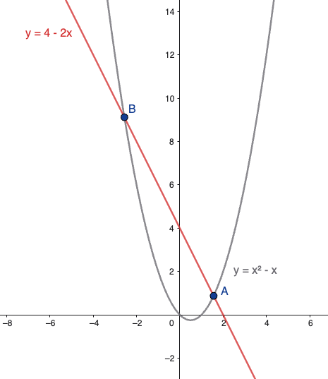
In particular, after graphing \(f(x)\) and \(g(x)\) separately, the graph itself shows that the parabola \(f(x)\) takes values greater than the line \(g(x)\) to the left of point \(B\) and to the right of point \(A\) (formally, for \(x<x_B\) or \(x>x_A\)).
The next step is to determine the x-coordinates of points \(A\) and \(B\) by solving the equation \(f(x)=g(x)\); substituting gives:
\[x^2-x=4-2x\]
and then, solving for \(x\) as follows, we obtain:
\[x^2+x-4=0\]
\[\Delta=(1)^2-4(1)(-4)=17\]
\[x_{A,B}=\frac{-1\pm\sqrt{17}}{2}\]
from which the solution of the inequality follows:
\[x<\frac{-1-\sqrt{17}}{2} \quad \text{or} \quad x>\frac{-1+\sqrt{17}}{2}\]
Example 3
Determine the solution of the following inequality graphically:
\[\sqrt{2x-2}<3\]
SOLUTION
As usual, the graphs of the two functions are drawn separately and then compared.
The function \(y=\sqrt{2x-2}\) represents the upper branch of a parabola with a horizontal axis and vertex \(V(1,0)\), lying in the first quadrant, while the function \(y=3\) represents a horizontal line. Fig. 7 shows the graphs of both functions drawn separately.
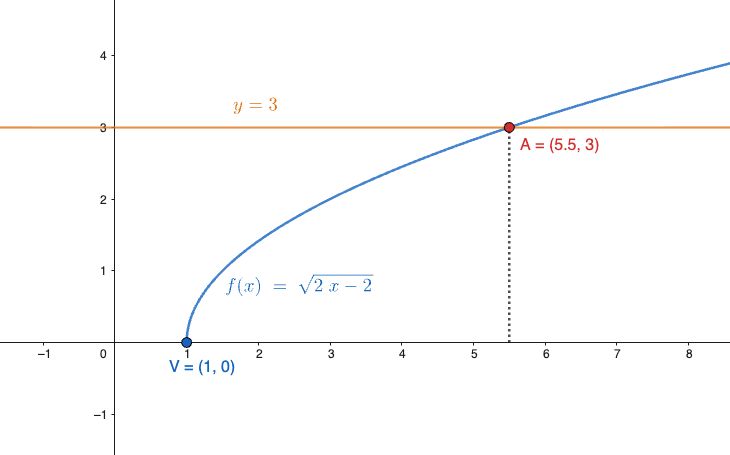
The problem requires \(y=\sqrt{2x-2}\) to be less than 3. This happens if and only if \(x\) lies between the vertex and the x-coordinate of point \(A\) (excluded), or, more rigorously, in the interval \(1\leq x<x_A\).
To go beyond the purely graphical aspect, the x-coordinate of \(A\) can be found analytically in a straightforward way as the intersection of the curve \(y=f(x)=\sqrt{2x-2}\) and the horizontal line \(y=3\); in formulas:
\[\sqrt{2x-2}=3\]
which, once solved (by squaring both sides), gives:
\[2x-2=9\]
\[2x=11\]
\[x_A=\frac{11}{2}=5.5\]
Common Mistakes
When equations and inequalities are solved graphically, attention must be paid to several recurring mistakes, which can lead to an incorrect solution set or to a misreading of the graph. Some common mistakes are listed below.
Confusing the intersection points with the solution set
For an equation, the solutions are the x-coordinates of the intersection points of the graphs of the functions involved. The points \((x,y)\) themselves are therefore not the solutions of the equation.
For example, if a parabola intersects the x-axis at the points \(A(x_1,0)\) and \(B(x_2,0)\), the solutions of the equation are
\[x=x_1 \qquad\text{and}\qquad x=x_2.\]
Overlooking the distinction between equations and inequalities
For an inequality, it is not enough to consider the intersection points of the graphs. The intervals of values of \(x\) on which one function is greater or less than the other must be identified.
In particular:
- \(f(x)>g(x)\) when the graph of \(f\) lies above the graph of \(g\);
- \(f(x)<g(x)\) when the graph of \(f\) lies below the graph of \(g\).
The intersection points are used instead to find the endpoints of the intervals.
Including the endpoints when the inequality is strict
A frequent mistake is to include the intersection points in the solutions of a strict inequality.
If the inequality is
\[f(x)>g(x)\]
or
\[f(x)<g(x),\]
the inequality is not satisfied at the points where \(f(x)=g(x)\). The endpoints of the intervals must therefore be excluded.
Conversely, for the inequalities
\[f(x)\ge g(x)\]
and
\[f(x)\le g(x),\]
the intersection points must be included.
Ignoring the domain of the function
Before a graph is interpreted, it must be checked that the function is actually defined on the interval considered.
This is particularly important for functions containing radicals. For example, for
\[f(x)=\sqrt{2x-2}\]
it must hold that
\[2x-2\ge0,\]
from which
\[x\ge1.\]
Consequently, values of \(x\) less than 1 cannot be considered, even if the graphical comparison might suggest doing so.
Squaring without checking the signs
When radicals appear in an equation or inequality, squaring both sides must be done with care.
For the equation
\[\sqrt{1-x^2}=\sqrt{x},\]
both sides are nonnegative, so squaring is legitimate. However, after the transformation, the constraints arising from the presence of the radicals must be kept.
In general, when algebraic manipulations may change the solution set, the domain restrictions should always be checked and, if necessary, the solutions obtained should be tested in the original equation.
Reversing the direction of the comparison
In a graphical comparison, attention must be paid to the direction of the inequality. If
\[f(x)>g(x),\]
the regions where the graph of \(f\) lies above that of \(g\) are to be considered; if instead
\[f(x)<g(x),\]
the regions where \(f\) lies below \(g\) are to be considered.
Reversing the comparison leads to exactly the wrong intervals.
Conclusion
The graphical method makes it possible to interpret equations and inequalities intuitively, turning an algebraic problem into a comparison between geometric objects. For quadratic equations, the solutions can be found by observing the intersections between the parabola and the x-axis, while for inequalities it is necessary to analyze the regions of the plane where the graph of the function satisfies the required comparison.
The graphical representation also makes the meaning of the discriminant immediately clear: the number of intersections between the parabola and the x-axis equals the number of real solutions of the equation.
The graphical method is particularly effective when the functions involved have a simple geometric representation, such as parabolas, lines, and circles. In more involved situations, the graph can be complemented by an analytical step, which is useful for determining precisely the coordinates of the intersection points and the endpoints of the solution intervals.
It is nevertheless important not to rely exclusively on a qualitative reading of the graph: the domain restrictions and the direction of the comparison must always be checked carefully. In this way, the graphical approach becomes not only a tool for finding the solutions but also an effective means of understanding their geometric meaning.
Final Test
The following test makes it possible to check understanding of the graphical method presented in this article. The questions range from the direct application of formulas to cases that require independent reasoning about the sign of the discriminant and the direction in which the parabola opens.
Cite this resource
"This page didn't write itself — every word here was written and checked by hand. If it helped you, sharing it or citing it as a source helps it reach the next student who needs it."
Citation
HTML link to copy