
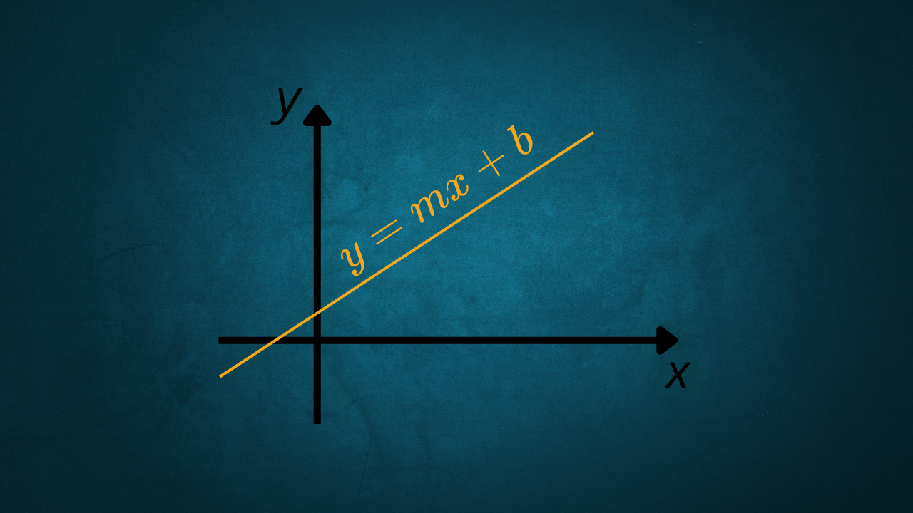
In mathematics, the line is one of the foundational topics of analytic geometry. This article covers how to recognize a line, represent it both geometrically and analytically, and write its equation in a clear, systematic way. The sections that follow work through every major aspect of the study of lines, with numerous examples.
No need to worry if lines, formulas, and graphs have felt confusing up to this point — every step here is built with logic and rigor, but explained clearly and accessibly.
With a bit of practice and the right method, it becomes possible to interpret the equation of a line and work through exercises with confidence, grasping both the algebraic and the geometric meaning behind each result.
What Is Analytic Geometry
Analytic geometry is the branch of mathematics that studies geometric figures using algebraic tools. The central idea is to associate a pair of values with every point in the plane, making it possible to describe geometric objects through equations; geometric problems can then be analyzed and solved with algebraic methods in a precise and general way.
Why the Line Is the Fundamental Object in Analytic Geometry
The line is the first and most important object in analytic geometry. It is simple from a geometric standpoint, yet extremely significant mathematically. Studying lines introduces foundational concepts such as slope, parallelism, perpendicularity, intersection, and more.
A solid understanding of the line also makes it possible to approach other areas of mathematics with greater confidence, not just analytic geometry.
Truly understanding the line means building a solid foundation: much of analytic geometry develops from this single object, directly or indirectly.
The Link Between Algebra, Analytic Geometry, and the Concept of a Line
In analytic geometry, every equation carries a geometric meaning, and every figure can be described by an equation. In the case of the line, this connection is immediate: a first-degree equation in two unknowns represents a line in the Cartesian plane.
⚠️ For many students, the main difficulty is not the computation but the interpretation: understanding what an equation represents and how to move from a geometric description to its algebraic expression.
Learning Objectives
By the end of this article, it will be possible to:
- understand the geometric meaning of the equation of a line in analytic geometry;
- recognize and use the different forms of the equation of a line;
- determine the equation of a line starting from geometric and/or analytic information;
- analyze the relative position of two or more lines in the plane;
- solve geometric problems using algebraic language.
Coordinate Axes and Lines Parallel to the Axes
Consider the Cartesian plane shown in Fig. 1:
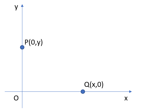
It is fairly clear that any point on the x-axis has generic coordinates Q(x, 0), which leads to the conclusion that this axis consists of all and only those points in the plane whose y-coordinate equals zero (y = 0).
In the same way, it is clear that the y-axis consists of all and only those points whose x-coordinate equals zero (x = 0).
In summary, the equations of the coordinate axes are:
y = 0 (equation of the x-axis)
x = 0 (equation of the y-axis)
In Fig. 2, consider the point P1 on the y-axis with generic coordinates (0, b), and draw a line parallel to the x-axis through that point. It becomes clear that the line (horizontal, shown in yellow) is the locus of all and only those points whose y-coordinate is constant and equal to b. Any point on it therefore has coordinates P(x, b).
This line has equation y = b.
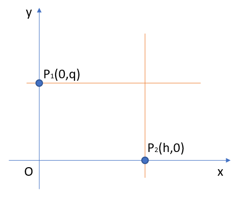
The same reasoning applies to the line parallel to the y-axis through P2, with coordinates (h, 0), lying on the x-axis (vertical line, shown in yellow): in analytic geometry, this line has equation x = h.
In summary, the equations of lines parallel to the coordinate axes are:
y = b (equation of a line parallel to the x-axis)
x = h (equation of a line parallel to the y-axis)
Slope of a Line and Its Geometric Interpretation
Definition of Slope
The slope of a generic line r is defined as the parameter m for which the ratio:
\[\frac{\Delta y}{\Delta x}\]
is constant.
In formulas:
\[m=\frac{\Delta y}{\Delta x}\tag{1}\]
In other words, the slope of a line represents the change in y-coordinate per unit change in x-coordinate.
Geometric Interpretation of Slope
From a geometric standpoint, the slope is directly tied to the inclination of a generic line r relative to the positive x-axis.
In other words, referring to Fig. 3, the slope, geometrically speaking, is the ratio between the lengths of segments BC and CA — with one important detail: these segments must always be treated as directed, since the slope can be either positive or negative.
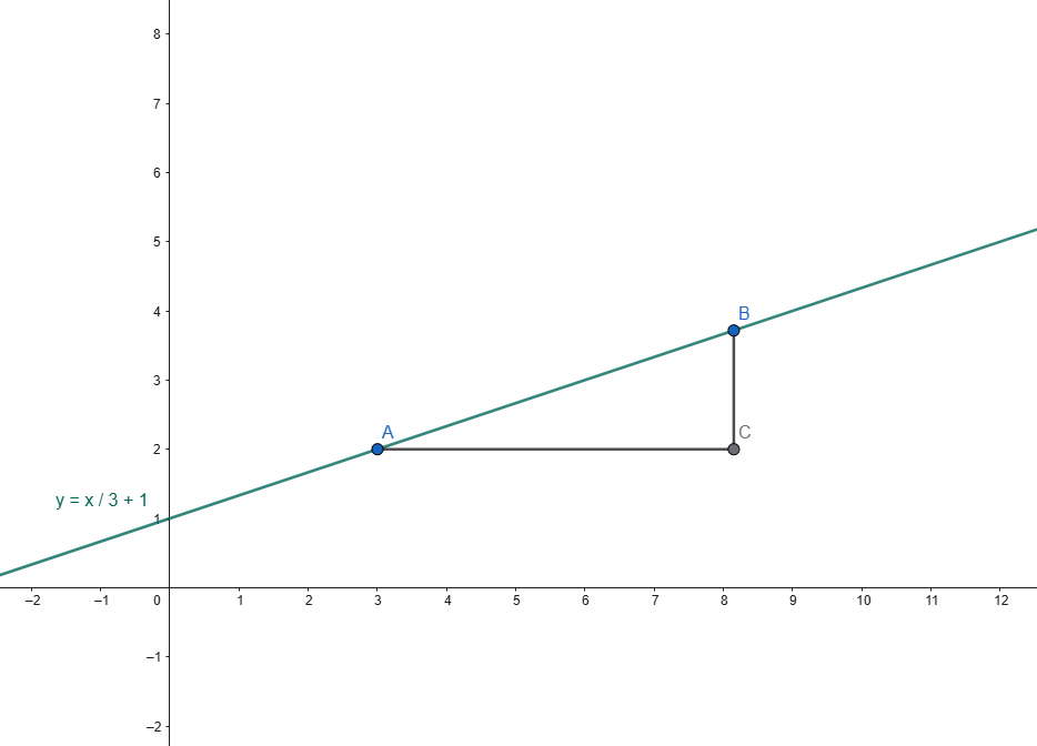
⚠️ Caution: it would not be correct to speak of a ratio of distances between points B and C and points A and C — since distances are always positive, that would always produce a ratio that is positive or, at most, zero. The slope, however, can also be negative.
Increasing, Decreasing, and Horizontal Lines
In the Cartesian plane, a line can have different inclinations depending on the value of the slope m, as shown in the following table:
| m > 0 | positive slope (increasing line) |
| m = 0 | zero slope (line parallel to the x-axis) |
| m < 0 | negative slope (decreasing line) |
| m undefined | line parallel to the y-axis |
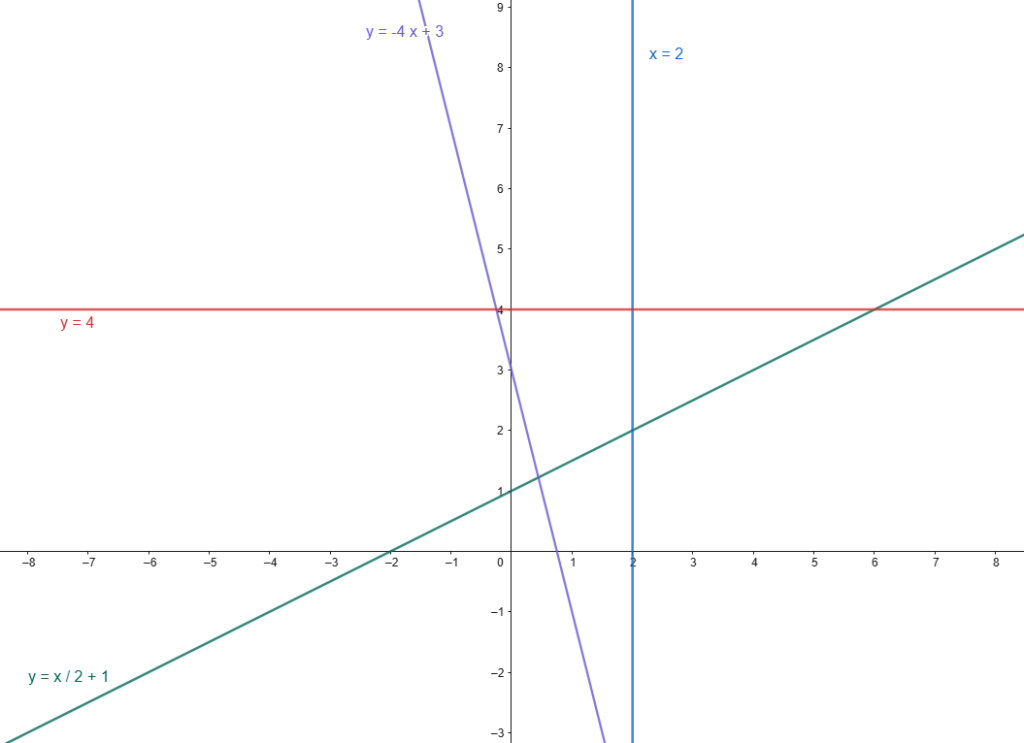
Let’s clarify this with some graphical examples and a summary table, using the lines shown in Fig. 4 below:
| Equation | Slope m | |
| y = x/2 + 1 | 1/2 (m > 0) | positive slope |
| y = 4 | m = 0 | zero slope (line parallel to the x-axis) |
| y = -4x + 3 | -4 (m < 0) | negative slope |
| x = 2 | m undefined | line parallel to the y-axis |
How the Graph of a Line Changes as the Slope Varies
The figure below (Fig. 5) shows how the graph of a line changes as the slope varies.
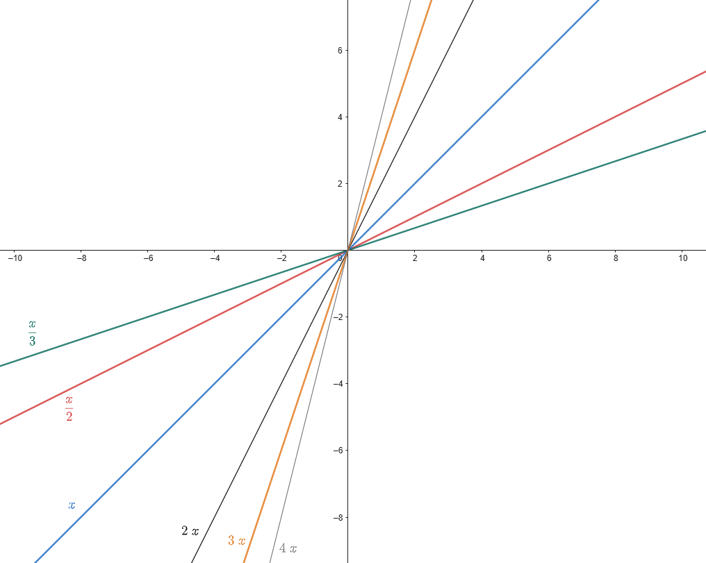
As the slope increases (positive values, in this example), the line’s steepness relative to the positive x-axis increases as well. In the figure, the line y = 4x (slope of 4) is the steepest of the group, while y = x/3 is the least steep.
For a deeper look at slope — including how to compute it from an angle of inclination and additional worked examples — see the dedicated article on the slope of a line.
Special Lines in the Cartesian Plane
Line Through the Origin
A line through the origin has an equation of the form:
\[y=mx\tag{2}\]
This equation represents the locus of points for which the y-coordinate is proportional to the x-coordinate, with a constant proportionality factor m, which corresponds to the slope.
Equation (2) clearly represents direct proportionality. To make the idea more concrete, consider a practical example.
EXAMPLE
Let m = 2. Equation (2) becomes:
y = 2x
and, for a few values of x (as shown in the table below), the corresponding values of y can be found. These values clearly show direct proportionality, and the proportionality factor is exactly the slope.
| x | -1 | 0 | 1 | 2 | 3 |
| y | -2 | 0 | 2 | 4 | 6 |
Equations of a Line in Analytic Geometry
Slope-Intercept Form of the Equation of a Line
The equation of a line in slope-intercept form can be written as:
\[y=mx+b\tag{3}\]
where \(m\) is the slope and \(b\) is the y-intercept.
This form is also known as the equation of a linear function (a rational, first-degree algebraic function).
General Form of the Equation of a Line
Any line in the plane can be represented, in the most general case, by the following equation, where the real coefficients a, b, and c can vary:
\[ax+by+c=0\tag{4}\]
Equation (4) is known as the general form of the equation of a line, where \(c\) denotes the constant term.
Let’s verify that every equation of this type represents a line.
Start with the following initial assumption:
\[a\neq 0\wedge b\neq 0\wedge c\neq 0\]
In this case, the general equation (4) can be rewritten as:
\[y=-\frac{a}{b}x-\frac{c}{b}\tag{5}\]
which represents the equation of a generic line with slope equal to:
\[m=-\frac{a}{b}\]
and y-intercept equal to:
\[y\text{-intercept}=-\frac{c}{b}\]
Geometrically, equation (5) represents a generic line in the plane that does not pass through the origin and is not parallel to either coordinate axis.
⚠️ Note: the coefficient b in the general form (4) is not the same quantity as the b used for the y-intercept in slope-intercept form (3) — the two equations use different coefficient sets, so b here refers strictly to the coefficient of y in ax + by + c = 0.
For a complete comparison of different forms of the equation of a line, see the dedicated article on the equation of a line: all forms explained.
Parallel and Perpendicular Lines
Condition for Parallel Lines
In analytic geometry, two lines (neither parallel to the y-axis) are said to be parallel if they have the same slope. Likewise, if two lines share the same slope, they are certainly parallel. In formulas:
\[r\parallel s\Leftrightarrow m_{r}=m_{s}\]
Recall that lines parallel to the x-axis have a slope of zero, while lines parallel to the y-axis have an undefined slope.
GRAPHICAL EXAMPLE of parallel lines (slope m = 1/2)
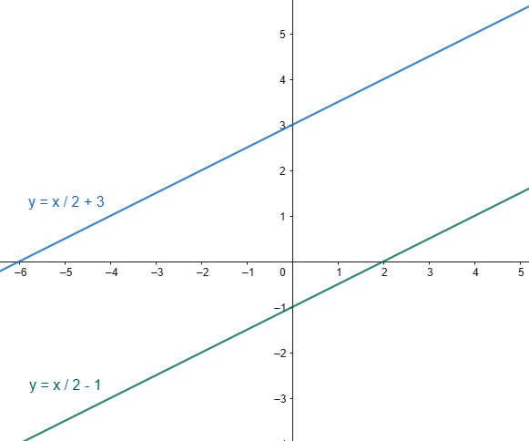
The lines shown in Fig. 6 above are clearly parallel to one another and share the same slope of 1/2.
Condition for Perpendicular Lines
Similar to the case of parallel lines just discussed, it is possible to define analytically a condition under which two lines are perpendicular to each other. The formal proof of perpendicularity between two lines will be covered in a dedicated article; for now, the focus is on the conceptual result and its practical application (being able to solve exercises).
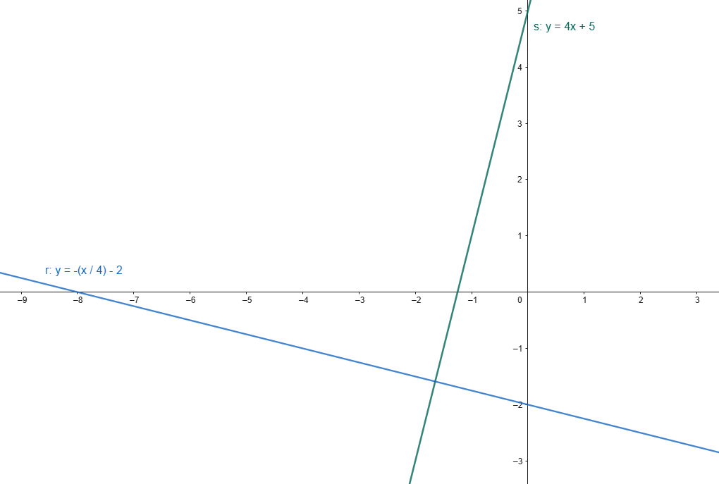
With that in mind, two lines, neither parallel to the axes, are perpendicular to each other if the product of their slopes equals -1 (equivalently, their slopes are opposite reciprocals of one another). This is also a necessary and sufficient condition.
In formulas:
\[ r\perp s\Leftrightarrow m_{r}\cdot m_{s}=-1\]
or, equivalently:
\[m_{r}=-\frac{1}{m_{s}}\]
Finally, if one of the two lines is parallel to the x-axis (say, line s), it will certainly have a slope of zero (ms = 0), while line r will have an undefined slope.
GRAPHICAL EXAMPLE of perpendicular lines (slope ms = 4 and mr = -1/4)
For a complete treatment of parallel and perpendicular lines, with additional worked examples, see the dedicated article on parallel and perpendicular lines.
Fundamental Equations of a Line
Equation of a Line Through a Point with a Given Slope
The equation of a line through a point with a known slope can be derived directly from the equation of a family of lines through a fixed point; it is simply a matter of assigning a specific value to the slope to obtain the desired line.
The equation of the line in this case takes the following form:
\[ y-y_{0}=m(x-x_{0})\tag{6}\]
with known slope \(m\).
EXAMPLE
Find the equation of line r with slope m = -2 passing through the point P0 with coordinates P0 = (4, 3).
Substituting the given values:
\[y-3=-2(x-4)\]
and simplifying:
\[y=-2x+11\]
which is the equation of the line.
For the special case of a line through a point that is parallel or perpendicular to another given line, see the dedicated article on finding a line through a point, parallel or perpendicular to a given line.
Slope of a Line Through Two Points
Consider points P and Q with coordinates P(x1, y1) and Q(x2, y2), such that the line r through P and Q is not parallel to the y-axis.
The slope of r is defined as the ratio between the difference in y-coordinates and the difference in x-coordinates of the two points, a direct application of equation (1). In formulas:
\[m=\frac{y_2-y_1}{x_2-x_1}\tag{7}\]
Notes:
- in this expression for \(m\), points P and Q are interchangeable — the formula can equally be written, without changing its meaning, as:
\[m=\frac{y_1-y_2}{x_1-x_2}\]
- the slope \(m\) can be found from knowledge of the two points P and Q alone, without needing to write the equation of the line through them.
EXAMPLE
Find the slope of the line through the points A(2, 3) and B(-2, 6).
Applying equation (7) to find \(m\):
\[m=\frac{6-3}{-2-2}=-\frac{3}{4}\]
Equation of a Line Through Two Points
This section covers how to correctly write the equation of a line through two given points P and Q.
Given two points in the Cartesian plane with coordinates P(x1, y1) and Q(x2, y2), chosen so that the line through them is parallel to neither the x-axis nor the y-axis, it can be shown that the line through these points can be written as:
\[\frac{y-y_{1}}{y_{2}-y_{1}}=\frac{x-x_{1}}{x_2-x_1}\tag{8}\]
EXAMPLE
Find the equation of the line through the points P(3, 6) and Q(-10, -1).
Using formula (8):
\[\frac{y-6}{-1-6}=\frac{x-3}{-10-3}\]
which gives
\[\frac{y-6}{-7}=\frac{x-3}{-13}\]
and, simplifying,
\[ 7x – 13y + 57 = 0 \]
which is the equation of the line (in general form) through points P and Q.
For a complete deep dive with fully worked examples and special cases, see the dedicated article on the equation of a line through two points.
Intercept Form of the Equation of a Line
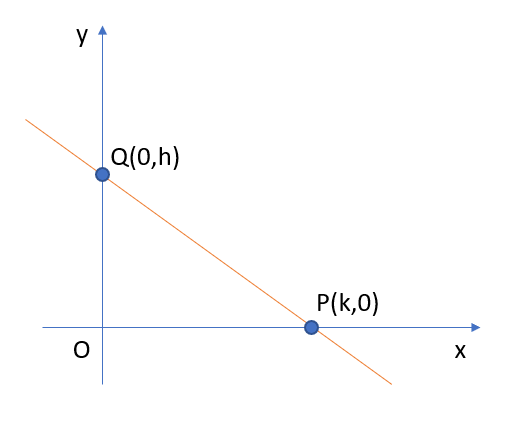
A special case, derived directly from the two-point equation of a line (8), arises when the two points lie on the coordinate axes — one on the x-axis, the other on the y-axis.
Suppose, for instance, that P lies on the x-axis: its generic coordinates can then be written as P(k, 0); likewise, suppose that Q lies on the y-axis, with generic coordinates Q(0, h).
Substituting these coordinates into equation (8):
\[\frac{y}{h}=\frac{x-k}{-k}\]
which, after distributing the denominator on the right-hand side and rearranging, immediately gives:
\[\frac{x}{k}+\frac{y}{h}=1\tag{9}\]
This is the intercept form of the equation of a line.
Distance From a Point to a Line
Many geometric applications require computing the distance from a point P(x0, y0) to a given line r. This distance is understood as the minimum distance from P to r.
It can be shown — with the full proof left to a dedicated article — that this distance can be expressed as:
\[ d=\frac{\left|ax_{0}+by_{0}+c\right|}{\sqrt{a^2+b^2}}\tag{10}\]
where r has equation
\[ax+by+c=0\]
Note: it can be shown that the segment representing the minimum distance between P and r meets the line at a right angle.
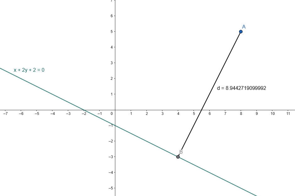
To make sense of this geometrically, consider a simple worked example.
WORKED EXAMPLE: DISTANCE FROM A POINT TO A LINE
Find the distance from point P to line r.
Given:
P(8, 5) → x0 = 8; y0 = 5
r: x + 2y + 2 = 0 → a = 1, b = 2, c = 2
\[d=\frac{1\cdot8+2\cdot 5+2}{\sqrt{1^2+2^2}}=\frac{20}{\sqrt{5}}\approx8.94427\]
To make the geometric meaning clearer, the result is shown in the Cartesian plane (Fig. 9):
For the distance of a line r from the origin O, formula (10) above reduces to:
\[ d=\frac{\left|c\right|}{\sqrt{a^2+b^2}}\tag{11}\]
since x0 = y0 = 0.
For a deeper look at the distance from a point to a line, with fully worked examples and proof, see the dedicated article on the distance from a point to a line.
Families of Lines in Analytic Geometry
The following section offers a brief overview of families of lines. For an in-depth look at the distinction between a family of parallel lines and a family of concurrent lines, with theory and guided exercises, see the full article on families of lines.
Family of Parallel Lines
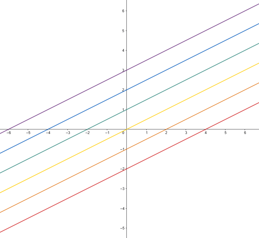
In analytic geometry, a family of parallel lines refers to the set of all lines in the plane sharing the same direction. These lines are therefore all parallel to one another and, as a result, all share the same slope m.
With m held constant, as the parameter k varies, the general equation of a family of parallel lines is:
\[y=mx+k\quad k\in\mathbb{R}\tag{12}\]
Note that for k = 0, the resulting line is the base line of the family, passing through the origin, to which every other line in the family is parallel as k varies.
⚠️ The equation above cannot be used to represent a family of lines parallel to the y-axis, since m is undefined in that case.
For that particular case, the family of lines parallel to the y-axis is described by the equation:
\[x=h\quad h\in\mathbb{R}\]
Family of Concurrent Lines
In analytic geometry, a family of concurrent lines consists of the set of lines in the Cartesian plane that share a common point, called point of concurrency, as the slope \(m\) varies.
Fig. 11 shows, as an example, a set of lines through the point C = (2, 3), which is the point of concurrency.
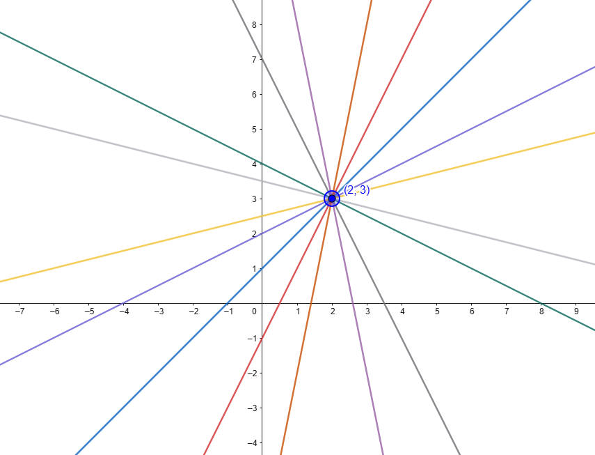
In general, to express analytically the equation of any line through the point of concurrency C, with known coordinates C = (x0, y0), the following formulation applies:
\[ y-y_{0}=m(x-x_{0})\tag{13}\]
as the slope m varies.
⚠️ Note that expression (13) cannot be used to describe the line parallel to the y-axis, since the slope is undefined in that case.
Geometric Loci in the Cartesian Plane
Definition of a Geometric Locus
Geometric loci are one of the foundational concepts in geometry, bridging the properties of individual points and the geometric figures that arise from them. This idea makes it possible to describe lines, curves, and surfaces not merely as drawings, but as sets of points satisfying precise geometric conditions. Understanding what a geometric locus is makes it possible to approach the study of figures such as the line (and beyond) with greater awareness, and to develop a rigorous method for solving geometric problems. This section covers what a geometric locus is, how to recognize one, and why it is such an important tool in the study of mathematics.
A geometric locus is the set of all and only those points of the plane (or of space) that satisfy a given geometric condition.
In other words:
- every point that satisfies the condition belongs to the geometric locus;
- no point that fails to satisfy it belongs to the locus.
For example, a circle is the geometric locus of points in the plane at a constant distance from a fixed point called the center.
This definition is fundamental to the study of geometry because it makes it possible to describe geometric figures through shared properties.
The concept of a geometric locus applies to lines as well.
In analytic geometry, a line can indeed be viewed as a geometric locus, since it is the set of all points satisfying a specific condition.
Examples
- The line through two points is the geometric locus of points collinear with two given points.
- The perpendicular bisector of a segment is the geometric locus of points that are equidistant from the endpoints of the segment.
- The line parallel to a given line through a point is the geometric locus of points that maintain a specific parallelism relationship.
Lines, curves, and surfaces in general can therefore all be interpreted as geometric loci, provided they are defined by a shared property of their points.
The next two sections focus on two specific types of geometric loci:
- the perpendicular bisector of a segment;
- the angle bisector.
Perpendicular Bisector of a Segment
As already mentioned, the perpendicular bisector of a segment can be defined as the locus of points equidistant from the endpoints of the segment.
Referring to Fig. 12, consider finding the equation of the perpendicular bisector of segment AB by applying the definition of a geometric locus.
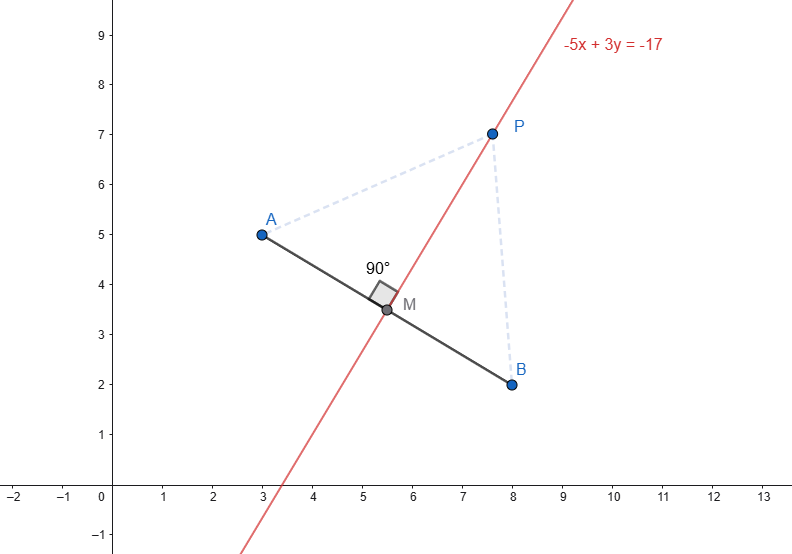
The coordinates of points A and B are known, and equal, respectively,
A(3, 5)
B(8, 2)
The equation of the perpendicular bisector of AB can be found by requiring it to be the locus of points for which the length of segment AP equals the length of segment BP, where P is a generic point with coordinates P(x, y). In formulas:
\[PA=PB\;\rightarrow\;PA^2=PB^2\]
and so, applying the formula for the distance between two points, in general:
\[ (x-x_1)^2 + (y-y_1)^2 = (x-x_2)^2 + (y-y_2)^2 \tag{14} \]
In this case:
\[(x-3)^2+(y-5)^2=(x-8)^2+(y-2)^2\]
which, once simplified, becomes, after working through the steps:
\( (x^2 – 6x + 9) + (y^2 – 10y + 25) \)
\( = \)
\( (x^2 – 16x + 64) + (y^2 – 4y + 4) \)
\( x^2 + y^2 – 6x – 10y + 34 \)
\( = \)
\( x^2 + y^2 – 16x – 4y + 68 \)
\( -6x – 10y + 34=-16x – 4y + 68 \)
\( 10x – 6y – 34 = 0 \)
\[ 5x – 3y – 17 = 0 \]
This final, simplified equation is that of a line — the geometric locus of points equidistant from:
A = (3, 5) and B = (8, 2).
Angle Bisector
This section covers another well-known geometric locus: the angle bisectors formed by two intersecting lines.
Consider two non-parallel lines r and s with equations
r: ax + by + c = 0
s: a’x + b’y + c’ = 0
Since an angle bisector consists of the locus of points equidistant from lines r and s, letting P(x, y) denote a generic point on the bisector, it follows that:
\( \frac{\left|ax+by+c\right|}{\sqrt{a^2+b^2}}=\frac{\left|a’x+b’y+c’\right|}{\sqrt{a’^2+b’^2}}\tag{15}\)
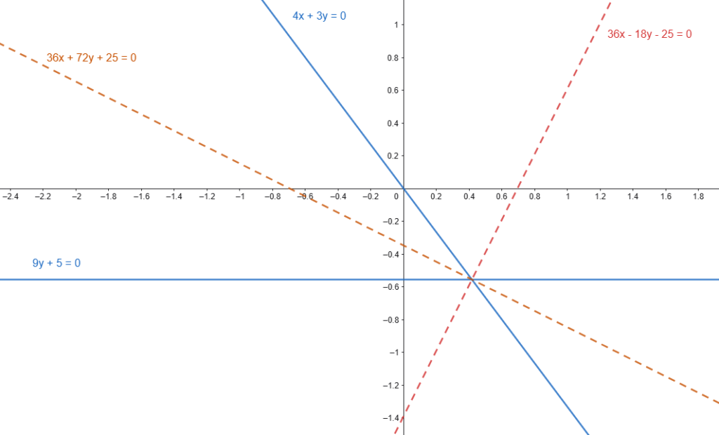
Equation (15) makes it possible to find the equations of the angle bisectors. Here’s a worked example.
EXAMPLE
Given the equations
r: 4x + 3y = 0
s: 9y + 5 = 0
find the equations of the bisectors of the angles formed by lines r and s.
Solution:
Applying (15):
\[ \frac{4x+3y}{\sqrt{4^2+3^2}} = \pm \frac{9y+5}{\sqrt{0^2+9^2}} \]
which gives
\[ \frac{4x+3y}{5} = \pm \frac{9y+5}{9}\]
and then
\[9(4x+3y) = \pm 5(9y+5) \]
Simplifying gives the equations of the two bisectors:
\[36x-18y-25=0\]
\[36x+72y+25=0\]
Parametric Equations of a Locus
Another way to derive the equation of a geometric locus is through parametric equations.
A system of parametric equations can generally be written in the form:
\[ \left\{ \begin{array}{l} x = f(t) \\ y = g(t) \end{array} \right. \qquad t \in \mathbb{R} \]
To find the equation of the locus in Cartesian form, the parameter t is eliminated from the system.
EXAMPLE
Find the Cartesian equation of the following geometric locus:
\[\left\{\begin{matrix}x=3t-1\\y=5t+2\end{matrix}\right.\;\;\;t\in \mathbb{R}\]
Solution
Isolate t from the first equation:
\( x = 3t – 1 \quad \Rightarrow \quad t = \frac{x+1}{3} \)
and substitute into the second:
\[ y = 5t + 2 = 5 \cdot \frac{x+1}{3} + 2 \]
and so:
\[ y = \frac{5x+5}{3} + \frac{6}{3} = \frac{5x+11}{3} \]
which is the equation of the line in explicit Cartesian form.
⚠️ Caution:
- Not every line can be written in slope-intercept form (vertical lines, \(x=k\), are one such case).
- Every line, however, can be written in general form.
Conclusion
The line is one of the foundational elements of analytic geometry and forms the basis for the topics that follow (e.g., the parabola, the circle, the ellipse, the hyperbola, and so on).
Through its different representations — slope-intercept, general, and parametric — this article has shown how to describe any line precisely and analytically, how to find the line through two given points, and how to identify lines parallel or perpendicular to a given line, and more.
The line is also a geometric locus, a set of points satisfying a linear relationship, and serves as the starting point for tackling more advanced concepts (e.g., angle bisectors).
Understanding the line is also essential for connecting to other topics in analytic geometry, such as the study of more complex geometric loci, the intersections between lines and curves, the extension of lines into three-dimensional space, and geometric transformations such as translations and rotations. In short, a solid grasp of the line makes it possible to tackle every subsequent topic in analytic geometry — and every related concept for which the line is an essential building block — with confidence and method.
For further practice applying these concepts, see the solved exercises on lines.
Cite this resource
"This page didn't write itself — every word here was written and checked by hand. If it helped you, sharing it or citing it as a source helps it reach the next student who needs it."
Citation
HTML link to copy